import matplotlib.pyplot as plt
import pandas as pd

from marine_qc import (
    Climatology,
    do_bayesian_buddy_check,
)

from data import get_climatology_data, get_grouped_data

How to use quality control checks with grouped reports

The marine_qc toolbox provides some quality control (QC) checks that work a group of marine reports. Creating some test dataset we can show how to use them on “real” data. There is one check that is shown here:

• a buddy check that tests that each observation is reasonably close to the average of its near neighbours in time and space

For more information of all available QC checks on a group of individual reports see the overview of QC functions for grouped reports.

The test dataset we provide is a pandas.DataFrame including marine reports representing the track of five ships. The QC functions return a QC flag for each individual report. The flags are:

• 0: the check has passed

• 1: the check has failed

• 2: the check is untestable

data = get_grouped_data()
data

	platform	date	lat	lon	sst
0	ship_1	2026-07-01 12:00:00	45.000914	-30.003120	19.612568
1	ship_1	2026-07-01 13:00:00	45.002822	-30.005853	23.977878
2	ship_1	2026-07-01 14:00:00	45.000384	-30.000949	19.670685
3	ship_1	2026-07-01 15:00:00	44.997441	-29.997362	19.616669
4	ship_1	2026-07-01 16:00:00	45.000198	-29.996618	19.396921
5	ship_1	2026-07-01 17:00:00	44.997422	-29.998894	19.182963
6	ship_2	2026-07-01 12:00:00	45.020635	-29.982150	19.472271
7	ship_2	2026-07-01 13:00:00	45.015957	-29.978332	19.650026
8	ship_2	2026-07-01 14:00:00	45.016715	-29.983056	24.253051
9	ship_2	2026-07-01 15:00:00	45.019096	-29.980762	19.564623
10	ship_2	2026-07-01 16:00:00	45.024425	-29.983219	19.249959
11	ship_2	2026-07-01 17:00:00	45.015559	-29.980152	19.496141
12	ship_3	2026-07-01 12:00:00	44.991658	-30.017520	19.376328
13	ship_3	2026-07-01 13:00:00	44.993952	-30.012770	19.754678
14	ship_3	2026-07-01 14:00:00	44.990003	-30.014304	19.690708
15	ship_3	2026-07-01 15:00:00	44.992656	-30.012386	24.033539
16	ship_3	2026-07-01 16:00:00	44.994037	-30.014797	19.370163
17	ship_3	2026-07-01 17:00:00	44.993894	-30.019371	19.278844
18	ship_4	2026-07-01 12:00:00	45.008589	-30.009917	19.458729
19	ship_4	2026-07-01 13:00:00	45.014485	-30.010597	19.818447
20	ship_4	2026-07-01 14:00:00	45.004951	-30.009005	19.697618
21	ship_4	2026-07-01 15:00:00	45.011759	-30.005866	19.619002
22	ship_4	2026-07-01 16:00:00	45.008954	-30.009387	23.955491
23	ship_4	2026-07-01 17:00:00	45.009426	-30.011827	19.156802
24	ship_5	2026-07-01 12:00:00	45.003242	-29.993509	19.521364
25	ship_5	2026-07-01 13:00:00	45.008071	-29.996282	19.696986
26	ship_5	2026-07-01 14:00:00	45.007877	-29.995928	19.741721
27	ship_5	2026-07-01 15:00:00	45.004014	-29.996089	19.442739
28	ship_5	2026-07-01 16:00:00	45.002412	-29.993539	19.256385
29	ship_5	2026-07-01 17:00:00	45.006037	-29.993558	23.893775

The ship data include six different parameters (lat, lon, date, and sst).

fig, (ax1, ax2) = plt.subplots(1, 2, figsize=(13, 5), constrained_layout=True)

colors = plt.cm.tab10.colors

i = 0
for color, (platform, group) in zip(colors, data.groupby("platform"), strict=False):
    ax1.plot(
        group["lon"],
        group["lat"],
        "-o",
        ms=5,
        label=platform,
        color=color,
    )

    ax2.plot(
        group["date"],
        group["sst"],
        "-o",
        ms=5,
        label=platform,
        color=color,
    )

    outlier = data.loc[(data.platform == platform) & (data.date == pd.Timestamp(f"2026-07-01 {13 + i}:00"))]

    ax1.scatter(
        outlier.lon,
        outlier.lat,
        s=150,
        facecolors="none",
        edgecolors="red",
        linewidth=2,
        zorder=10,
    )

    ax2.scatter(
        outlier.date,
        outlier.sst,
        s=150,
        facecolors="none",
        edgecolors="red",
        linewidth=2,
        zorder=10,
    )

    i += 1

ax1.set_xlabel("Longitude (°)")
ax1.set_ylabel("Latitude (°)")
ax1.set_title("Buddy observations")
ax1.legend(loc="best")

ax2.set_xlabel("Time")
ax2.set_ylabel("SST (°C)")
ax2.set_title("Sea surface temperature")
ax2.tick_params(axis="x", rotation=30)

plt.show()

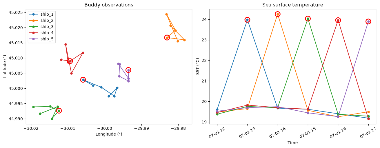
We see five different ships. Each of them includes one value that is much higher than the others. These values should be detected and flagged as 1 (failed).

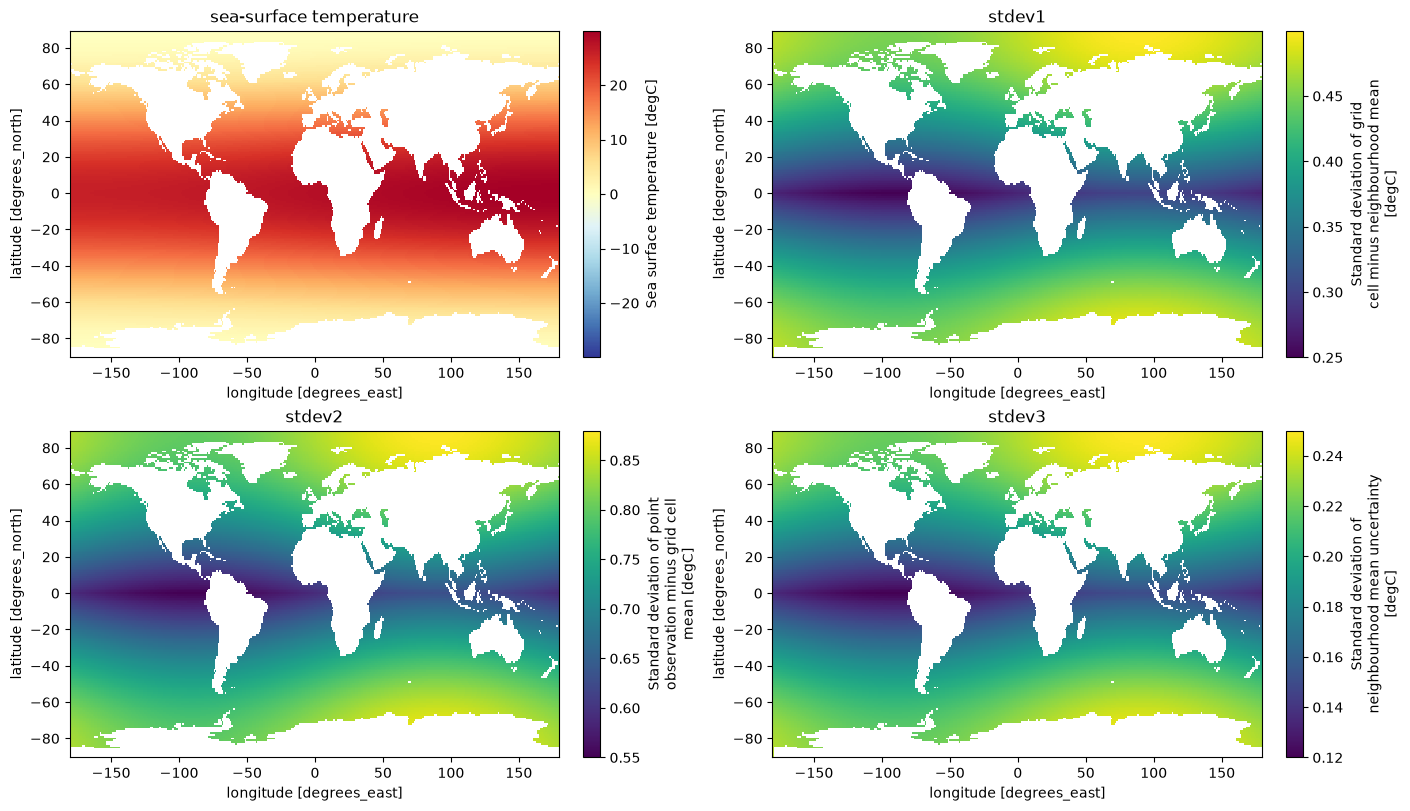
Firtly, we import some external data. This is a xarray.Dataset containing CF-compliant data:

• a land-sea mask where 1 denotes a land point and 0 denotes a sea point (land_sea_mask)

• a simple, latitudinally and longitudinally dependent sea-surface temperature field (sst)

• a sea-surface temperature standard deviation of grid cell minus neighbourhood mean (sst_stde1)

• a sea-surface temperature standard deviation of point observation minus grid cell mean (sst_stde2)

• a sea-surface temperature standard deviation of neighbourhood mean uncertainty (sst_stde3)

climatology_data = get_climatology_data()
climatology_data

/home/docs/checkouts/readthedocs.org/user_builds/marine-qc/conda/latest/lib/python3.14/site-packages/cartopy/io/__init__.py:242: DownloadWarning: Downloading: https://naturalearth.s3.amazonaws.com/110m_physical/ne_110m_land.zip
  warnings.warn(f'Downloading: {url}', DownloadWarning)

<xarray.Dataset> Size: 2MB
Dimensions:        (time: 1, latitude: 180, longitude: 360)
Coordinates:
  * time           (time) datetime64[us] 8B 2026-07-01T12:00:00
  * latitude       (latitude) int64 1kB -90 -89 -88 -87 -86 ... 85 86 87 88 89
  * longitude      (longitude) int64 3kB -180 -179 -178 -177 ... 176 177 178 179
Data variables:
    land_sea_mask  (time, latitude, longitude) int8 65kB 0 1 1 1 1 ... 0 0 0 0 0
    sst            (time, latitude, longitude) float64 518kB -1.225e-16 ... 0...
    sst_stdev1     (time, latitude, longitude) float64 518kB 0.475 ... 0.4754
    sst_stdev2     (time, latitude, longitude) float64 518kB 0.84 nan ... 0.8407
    sst_stdev3     (time, latitude, longitude) float64 518kB 0.235 ... 0.2352
    crs            int64 8B 0

xarray.Dataset

• Dimensions:
  • time: 1
  • latitude: 180
  • longitude: 360
• Coordinates: (3)
  • time
    (time)
    datetime64[us]
    2026-07-01T12:00:00

    standard_name :

    time

    axis :

    T

    array(['2026-07-01T12:00:00.000000'], dtype='datetime64[us]')

  • latitude
    (latitude)
    int64
    -90 -89 -88 -87 -86 ... 86 87 88 89

    standard_name :

    latitude

    units :

    degrees_north

    axis :

    Y

    array([-90, -89, -88, -87, -86, -85, -84, -83, -82, -81, -80, -79, -78, -77,
           -76, -75, -74, -73, -72, -71, -70, -69, -68, -67, -66, -65, -64, -63,
           -62, -61, -60, -59, -58, -57, -56, -55, -54, -53, -52, -51, -50, -49,
           -48, -47, -46, -45, -44, -43, -42, -41, -40, -39, -38, -37, -36, -35,
           -34, -33, -32, -31, -30, -29, -28, -27, -26, -25, -24, -23, -22, -21,
           -20, -19, -18, -17, -16, -15, -14, -13, -12, -11, -10,  -9,  -8,  -7,
            -6,  -5,  -4,  -3,  -2,  -1,   0,   1,   2,   3,   4,   5,   6,   7,
             8,   9,  10,  11,  12,  13,  14,  15,  16,  17,  18,  19,  20,  21,
            22,  23,  24,  25,  26,  27,  28,  29,  30,  31,  32,  33,  34,  35,
            36,  37,  38,  39,  40,  41,  42,  43,  44,  45,  46,  47,  48,  49,
            50,  51,  52,  53,  54,  55,  56,  57,  58,  59,  60,  61,  62,  63,
            64,  65,  66,  67,  68,  69,  70,  71,  72,  73,  74,  75,  76,  77,
            78,  79,  80,  81,  82,  83,  84,  85,  86,  87,  88,  89])

  • longitude
    (longitude)
    int64
    -180 -179 -178 -177 ... 177 178 179

    standard_name :

    longitude

    units :

    degrees_east

    axis :

    X

    array([-180, -179, -178, ...,  177,  178,  179], shape=(360,))

• Data variables: (6)
  • land_sea_mask
    (time, latitude, longitude)
    int8
    0 1 1 1 1 1 1 1 ... 0 0 0 0 0 0 0 0

    long_name :

    Land-sea mask

    flag_values :

    [0 1]

    flag_meanings :

    land sea

    coordinates :

    latitude longitude time

    array([[[0, 1, 1, ..., 1, 1, 1],
            [0, 1, 1, ..., 1, 1, 1],
            [0, 1, 1, ..., 1, 1, 1],
            ...,
            [0, 0, 0, ..., 0, 0, 0],
            [0, 0, 0, ..., 0, 0, 0],
            [0, 0, 0, ..., 0, 0, 0]]], shape=(1, 180, 360), dtype=int8)

  • sst
    (time, latitude, longitude)
    float64
    -1.225e-16 nan ... 0.04343 0.04343

    standard_name :

    sea_surface_temperature

    long_name :

    Sea surface temperature

    units :

    degC

    coordinates :

    time latitude longitude

    grid_mapping :

    crs

    array([[[-1.22464680e-16,             nan,             nan, ...,
                         nan,             nan,             nan],
            [-2.63763911e-02,             nan,             nan, ...,
                         nan,             nan,             nan],
            [-3.56956970e-02,             nan,             nan, ...,
                         nan,             nan,             nan],
            ...,
            [-2.79784476e-02, -2.79744621e-02, -2.79625056e-02, ...,
              1.81329509e-01,  1.81349435e-01,  1.81361392e-01],
            [-3.56956970e-02, -3.56930393e-02, -3.56850663e-02, ...,
              1.03878371e-01,  1.03891659e-01,  1.03899632e-01],
            [-2.63763911e-02, -2.63750621e-02, -2.63710750e-02, ...,
              4.34212736e-02,  4.34279184e-02,  4.34319055e-02]]],
          shape=(1, 180, 360))

  • sst_stdev1
    (time, latitude, longitude)
    float64
    0.475 nan nan ... 0.4758 0.4754

    units :

    degC

    coordinates :

    time latitude longitude

    grid_mapping :

    crs

    long_name :

    Standard deviation of grid cell minus neighbourhood mean

    array([[[0.475     ,        nan,        nan, ...,        nan,
                    nan,        nan],
            [0.47496954,        nan,        nan, ...,        nan,
                    nan,        nan],
            [0.47487817,        nan,        nan, ...,        nan,
                    nan,        nan],
            ...,
            [0.47472591, 0.4742896 , 0.47385342, ..., 0.47603431,
             0.47559839, 0.47516222],
            [0.47487817, 0.47444186, 0.47400568, ..., 0.47618656,
             0.47575065, 0.47531448],
            [0.47496954, 0.47453323, 0.47409705, ..., 0.47627794,
             0.47584203, 0.47540585]]], shape=(1, 180, 360))

  • sst_stdev2
    (time, latitude, longitude)
    float64
    0.84 nan nan ... 0.8414 0.8407

    units :

    degC

    coordinates :

    time latitude longitude

    grid_mapping :

    crs

    long_name :

    Standard deviation of point observation minus grid cell mean

    array([[[0.84      ,        nan,        nan, ...,        nan,
                    nan,        nan],
            [0.83996192,        nan,        nan, ...,        nan,
                    nan,        nan],
            [0.83984771,        nan,        nan, ...,        nan,
                    nan,        nan],
            ...,
            [0.83965738, 0.83895929, 0.8382614 , ..., 0.84175082,
             0.84105336, 0.84035548],
            [0.83984771, 0.83914961, 0.83845173, ..., 0.84194115,
             0.84124369, 0.8405458 ],
            [0.83996192, 0.83926383, 0.83856594, ..., 0.84205536,
             0.8413579 , 0.84066002]]], shape=(1, 180, 360))

  • sst_stdev3
    (time, latitude, longitude)
    float64
    0.235 nan nan ... 0.2355 0.2352

    units :

    degC

    coordinates :

    time latitude longitude

    grid_mapping :

    crs

    long_name :

    Standard deviation of neighbourhood mean uncertainty

    array([[[0.235     ,        nan,        nan, ...,        nan,
                    nan,        nan],
            [0.23498477,        nan,        nan, ...,        nan,
                    nan,        nan],
            [0.23493908,        nan,        nan, ...,        nan,
                    nan,        nan],
            ...,
            [0.23486295, 0.23460117, 0.23433946, ..., 0.23564799,
             0.23538645, 0.23512474],
            [0.23493908, 0.2346773 , 0.23441559, ..., 0.23572412,
             0.23546258, 0.23520087],
            [0.23498477, 0.23472298, 0.23446128, ..., 0.23576981,
             0.23550826, 0.23524656]]], shape=(1, 180, 360))

  • crs
    ()
    int64
    0

    grid_mapping_name :

    latitude_longitude

    epsg_code :

    EPSG:4326

    semi_major_axis :

    6378137.0

    inverse_flattening :

    298.257223563

    array(0)

For the buddy check, we need some external data:

• climatology: The climatological average(s) used to calculate anomalies.

• stdev1: Field of standard deviations representing standard deviation of difference between target gridcell and complete neighbour average (grid area to neighbourhood difference)

• stdev2: Field of standard deviations representing standard deviation of difference between a single observation and the target gridcell average (point to grid area difference)

• stdev3: Field of standard deviations representing standard deviation of difference between random neighbour gridcell and full neighbour average (uncertainty in neighbour average)

fig, axes = plt.subplots(
    2,
    2,
    figsize=(14, 8),
    constrained_layout=True,
)

plots = [
    ("sst", "sea-surface temperature", "RdYlBu_r"),
    ("sst_stdev1", "stdev1", "viridis"),
    ("sst_stdev2", "stdev2", "viridis"),
    ("sst_stdev3", "stdev3", "viridis"),
]

for ax, (var, title, cmap) in zip(axes.flat, plots, strict=False):
    climatology_data[var].isel(time=0).plot(
        ax=ax,
        cmap=cmap,
        add_colorbar=True,
    )
    ax.set_title(title)

plt.show()

Unfortunately, the standard deviations have to be converted manually to marine_qc.Climatology classes.

sst_stdev1 = Climatology(climatology_data.sst_stdev1)
sst_stdev2 = Climatology(climatology_data.sst_stdev2)
sst_stdev3 = Climatology(climatology_data.sst_stdev3)

Besiedes the external climatologies some additional parameters needs to be set:

• prior_probability_of_gross_error: prior probability of gross error, which is the background rate of gross errors (0.05)

• quantization_interval: smallest possible increment in the input values (0.1)

• one_sigma_measurement_uncertainty: estimated one sigma measurement uncertainty (1.0)

• limits: list with three members which specify the search range for the buddy check ([2, 2, 4])

• noise_scaling: tuning parameter used to multiply stdev2 (3.0)

• maximum_anomaly: largest absolute anomaly, assumes that the maximum and minimum anomalies have the same magnitude (8.0)

• fail_probability: probability of gross error that corresponds to a failed test. Anything with a probability of gross error greater than fail_probability will be considered failing (0.3)

qc_buddy = do_bayesian_buddy_check(
    value=data.sst,
    lat=data.lat,
    lon=data.lon,
    date=data.date,
    climatology=climatology_data.sst,
    stdev1=sst_stdev1,
    stdev2=sst_stdev2,
    stdev3=sst_stdev3,
    prior_probability_of_gross_error=0.05,
    quantization_interval=0.1,
    one_sigma_measurement_uncertainty=1.0,
    limits=[2, 2, 4],
    noise_scaling=3.0,
    maximum_anomaly=8.0,
    fail_probability=0.3,
)
pd.DataFrame({**data, "qc_flag": qc_buddy})

	platform	date	lat	lon	sst	qc_flag
0	ship_1	2026-07-01 12:00:00	45.000914	-30.003120	19.612568	0
1	ship_1	2026-07-01 13:00:00	45.002822	-30.005853	23.977878	1
2	ship_1	2026-07-01 14:00:00	45.000384	-30.000949	19.670685	0
3	ship_1	2026-07-01 15:00:00	44.997441	-29.997362	19.616669	0
4	ship_1	2026-07-01 16:00:00	45.000198	-29.996618	19.396921	0
5	ship_1	2026-07-01 17:00:00	44.997422	-29.998894	19.182963	0
6	ship_2	2026-07-01 12:00:00	45.020635	-29.982150	19.472271	0
7	ship_2	2026-07-01 13:00:00	45.015957	-29.978332	19.650026	0
8	ship_2	2026-07-01 14:00:00	45.016715	-29.983056	24.253051	1
9	ship_2	2026-07-01 15:00:00	45.019096	-29.980762	19.564623	0
10	ship_2	2026-07-01 16:00:00	45.024425	-29.983219	19.249959	0
11	ship_2	2026-07-01 17:00:00	45.015559	-29.980152	19.496141	0
12	ship_3	2026-07-01 12:00:00	44.991658	-30.017520	19.376328	0
13	ship_3	2026-07-01 13:00:00	44.993952	-30.012770	19.754678	0
14	ship_3	2026-07-01 14:00:00	44.990003	-30.014304	19.690708	0
15	ship_3	2026-07-01 15:00:00	44.992656	-30.012386	24.033539	1
16	ship_3	2026-07-01 16:00:00	44.994037	-30.014797	19.370163	0
17	ship_3	2026-07-01 17:00:00	44.993894	-30.019371	19.278844	0
18	ship_4	2026-07-01 12:00:00	45.008589	-30.009917	19.458729	0
19	ship_4	2026-07-01 13:00:00	45.014485	-30.010597	19.818447	0
20	ship_4	2026-07-01 14:00:00	45.004951	-30.009005	19.697618	0
21	ship_4	2026-07-01 15:00:00	45.011759	-30.005866	19.619002	0
22	ship_4	2026-07-01 16:00:00	45.008954	-30.009387	23.955491	1
23	ship_4	2026-07-01 17:00:00	45.009426	-30.011827	19.156802	0
24	ship_5	2026-07-01 12:00:00	45.003242	-29.993509	19.521364	0
25	ship_5	2026-07-01 13:00:00	45.008071	-29.996282	19.696986	0
26	ship_5	2026-07-01 14:00:00	45.007877	-29.995928	19.741721	0
27	ship_5	2026-07-01 15:00:00	45.004014	-29.996089	19.442739	0
28	ship_5	2026-07-01 16:00:00	45.002412	-29.993539	19.256385	0
29	ship_5	2026-07-01 17:00:00	45.006037	-29.993558	23.893775	1

We get the expected results.