import matplotlib.pyplot as plt

import pandas as pd

from marine_qc import (
    combine_qc_results,
    do_iquam_track_check,
    do_multiple_sequential_check,
    do_spike_check,
)

from data import get_sequential_data

How to use quality control checks with sequential reports from ships¶

The marine_qc toolbox provides some quality control (QC) checks that work on sequential marine ship reports. Creating some test dataset we can show how to use them on “real” data. There are two checks that are shown here:

a spike check that tests that a sequence of values has unlikely “spikes” in it.
a track check that tests that the locations of a series of reports form a plausible ship track

Finally, we run all these QC checks within a single function and combine the results of each QC check into a single QC flag.

For more information of all available QC checks on sequential ship reports see the overview of QC functions for sequential ship reports.

The test dataset we provide is a pandas.DataFrame including sequential marine reports representing the track of one ship. The QC functions return a QC flag for each individual report. The flags are:

0: the check has passed
1: the check has failed
2: the check is untestable

data = get_sequential_data()
data

	ship_id	date	lat	lon	sst
0	ship_1	2026-07-01 00:00:00	44.919061	-29.771070	20.270235
1	ship_1	2026-07-01 01:00:00	44.814792	-29.530290	35.399830
2	ship_1	2026-07-01 02:00:00	44.688881	-29.278467	20.527780
3	ship_1	2026-07-01 03:00:00	44.544855	-29.017162	20.646629
4	ship_1	2026-07-01 04:00:00	44.387443	-28.748580	20.749549
5	ship_1	2026-07-01 05:00:00	44.221920	-28.475424	20.830890
6	ship_1	2026-07-01 06:00:00	44.053692	-28.200708	20.886577
7	ship_1	2026-07-01 07:00:00	43.888168	-27.927552	20.914328
8	ship_1	2026-07-01 08:00:00	43.730756	-27.658971	20.913721
9	ship_1	2026-07-01 09:00:00	43.586731	-27.397665	20.886160
10	ship_1	2026-07-01 10:00:00	43.460819	-27.145842	20.834795
11	ship_1	2026-07-01 11:00:00	43.356550	-26.905062	20.764390
12	ship_1	2026-07-01 12:00:00	43.275611	-26.676132	20.681097
13	ship_1	2026-07-01 13:00:00	43.217526	-26.459053	20.592091
14	ship_1	2026-07-01 14:00:00	43.179818	-26.253016	20.505045
15	ship_1	2026-07-01 15:00:00	43.158587	-26.056461	20.427510
16	ship_1	2026-07-01 16:00:00	43.149206	-25.867183	35.366288
17	ship_1	2026-07-01 17:00:00	43.146876	-25.682479	20.326911
18	ship_1	2026-07-01 18:00:00	43.146876	-25.499335	20.313281
19	ship_1	2026-07-01 19:00:00	43.144546	-25.314631	35.327493
20	ship_1	2026-07-01 20:00:00	43.135165	-25.125353	20.369799
21	ship_1	2026-07-01 21:00:00	43.113934	-24.928799	20.438674
22	ship_1	2026-07-01 22:00:00	43.076227	-24.722762	20.530943
23	ship_1	2026-07-01 23:00:00	43.018141	-24.505682	20.641937

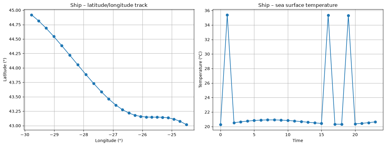
The ship data include four different parameters (lat, lon, date, and sst).

fig, axs = plt.subplots(1, 2, figsize=(13, 5))

axs[0].plot(data["lon"], data["lat"], marker="o", linestyle="-")
axs[0].set_title("Ship – latitude/longitude track")
axs[0].set_xlabel("Longitude (°)")
axs[0].set_ylabel("Latitude (°)")
axs[0].grid(True)

axs[1].plot(data["sst"], marker="o", linestyle="-")
axs[1].set_title("Ship – sea surface temperature")
axs[1].set_xlabel("Time")
axs[1].set_ylabel("Temperature (°C)")
axs[1].grid(True)

plt.tight_layout()
plt.show()

../_images/34ad2c27a06e10359dda41fa6ef6d23a3412489cc667c7a37188ddbed8109118.png

Firstly, a spike check is performed. Beside lat, lon, date and value, this check needs some extra parameters:

max_gradient_space: Maximum allowed spatial gradient (0.5: “0.5 K per kilometer”)
max_gradient_time: Maximum allowed temporal gradient (1.0: “1.0 K per kilometer”)
delta_t: Temperature delta used in the comparison (2.0: “2.0 K”)
n_neighbours: Number of neighboring points considered in the analysis (5)

qc_spike = do_spike_check(
    value=data.sst,
    lat=data.lat,
    lon=data.lon,
    date=data.date,
    max_gradient_space=0.5,
    max_gradient_time=1.0,
    delta_t=2.0,
    n_neighbours=5,
)
pd.DataFrame({"lat": data.lat, "lon": data.lon, "date": data.date, "sst": data.sst, "qc_spike": qc_spike})

	lat	lon	date	sst	qc_spike
0	44.919061	-29.771070	2026-07-01 00:00:00	20.270235	0
1	44.814792	-29.530290	2026-07-01 01:00:00	35.399830	1
2	44.688881	-29.278467	2026-07-01 02:00:00	20.527780	0
3	44.544855	-29.017162	2026-07-01 03:00:00	20.646629	0
4	44.387443	-28.748580	2026-07-01 04:00:00	20.749549	0
5	44.221920	-28.475424	2026-07-01 05:00:00	20.830890	0
6	44.053692	-28.200708	2026-07-01 06:00:00	20.886577	0
7	43.888168	-27.927552	2026-07-01 07:00:00	20.914328	0
8	43.730756	-27.658971	2026-07-01 08:00:00	20.913721	0
9	43.586731	-27.397665	2026-07-01 09:00:00	20.886160	0
10	43.460819	-27.145842	2026-07-01 10:00:00	20.834795	0
11	43.356550	-26.905062	2026-07-01 11:00:00	20.764390	0
12	43.275611	-26.676132	2026-07-01 12:00:00	20.681097	0
13	43.217526	-26.459053	2026-07-01 13:00:00	20.592091	0
14	43.179818	-26.253016	2026-07-01 14:00:00	20.505045	0
15	43.158587	-26.056461	2026-07-01 15:00:00	20.427510	0
16	43.149206	-25.867183	2026-07-01 16:00:00	35.366288	1
17	43.146876	-25.682479	2026-07-01 17:00:00	20.326911	0
18	43.146876	-25.499335	2026-07-01 18:00:00	20.313281	0
19	43.144546	-25.314631	2026-07-01 19:00:00	35.327493	1
20	43.135165	-25.125353	2026-07-01 20:00:00	20.369799	0
21	43.113934	-24.928799	2026-07-01 21:00:00	20.438674	0
22	43.076227	-24.722762	2026-07-01 22:00:00	20.530943	0
23	43.018141	-24.505682	2026-07-01 23:00:00	20.641937	0

In the plot above, we can see three obvious spikes that are represented in the results of the spike check (1 (failed)). The spike checks gives the expected results.

Now, we do the track check. As for the spike check we need some extra parameters:

speed_limit: Speed limit of platform in kilometers per hour (25.0)
delta_d: Latitude tolerance in degrees (1.11)
delta_t: Time tolerance in hundredths of an hour (0.01)
n_neighbours: Number of neighbouring points considered in the analysis (5)

qc_track = do_iquam_track_check(
    lat=data.lat,
    lon=data.lon,
    date=data.date,
    speed_limit=25.0,
    delta_d=1.11,
    delta_t=0.01,
    n_neighbours=5,
)
pd.DataFrame({"lat": data.lat, "lon": data.lon, "date": data.date, "qc_track": qc_track})

	lat	lon	date	qc_track
0	44.919061	-29.771070	2026-07-01 00:00:00	0
1	44.814792	-29.530290	2026-07-01 01:00:00	0
2	44.688881	-29.278467	2026-07-01 02:00:00	0
3	44.544855	-29.017162	2026-07-01 03:00:00	0
4	44.387443	-28.748580	2026-07-01 04:00:00	1
5	44.221920	-28.475424	2026-07-01 05:00:00	1
6	44.053692	-28.200708	2026-07-01 06:00:00	1
7	43.888168	-27.927552	2026-07-01 07:00:00	1
8	43.730756	-27.658971	2026-07-01 08:00:00	1
9	43.586731	-27.397665	2026-07-01 09:00:00	0
10	43.460819	-27.145842	2026-07-01 10:00:00	0
11	43.356550	-26.905062	2026-07-01 11:00:00	0
12	43.275611	-26.676132	2026-07-01 12:00:00	0
13	43.217526	-26.459053	2026-07-01 13:00:00	0
14	43.179818	-26.253016	2026-07-01 14:00:00	0
15	43.158587	-26.056461	2026-07-01 15:00:00	0
16	43.149206	-25.867183	2026-07-01 16:00:00	0
17	43.146876	-25.682479	2026-07-01 17:00:00	0
18	43.146876	-25.499335	2026-07-01 18:00:00	0
19	43.144546	-25.314631	2026-07-01 19:00:00	0
20	43.135165	-25.125353	2026-07-01 20:00:00	0
21	43.113934	-24.928799	2026-07-01 21:00:00	0
22	43.076227	-24.722762	2026-07-01 22:00:00	0
23	43.018141	-24.505682	2026-07-01 23:00:00	0

Within the given parameters, the ship is too “fast” between (44.387443, -28.748580) and (43.730756, -27.658971).

Now, we can run these two QC checks within a single function do_multiple_sequential_check. Therefore, we need a pandas.DataFrame and a nested QC dictionary. This is the structure of the dictionary:

arbitrary user-specified name for the checks
- “func”: name of the QC function as str (mandatory)
- “names”: dictionary containing parameter names of the QC function and their corresponding columns in the pandas.DataFrame (mandatory)
- “arguments”: dictionary containing any key-word arguments passed to the QC function (optionally)
…

We define the QC dictionary according to the QC checks above.

qc_dict = {
    "spike_check": {
        "func": "do_spike_check",
        "names": {
            "value": "sst",
            "lat": "lat",
            "lon": "lon",
            "date": "date",
        },
        "arguments": {
            "max_gradient_space": 0.5,
            "max_gradient_time": 1.0,
            "delta_t": 1.0,
            "n_neighbours": 5,
        },
    },
    "iquam_track_check": {
        "func": "do_iquam_track_check",
        "names": {
            "lat": "lat",
            "lon": "lon",
            "date": "date",
        },
        "arguments": {
            "speed_limit": 25.0,
            "delta_d": 1.11,
            "delta_t": 0.01,
            "n_neighbours": 5,
        },
    },
}

We set return_method to “failed” which means that all requested QC check are run until the first check fails. The other QC checks are flagged as unstested (3). Furthermore, we set groupby to “ship_id” which specifies how the data should be grouped before applying QC functions.

qc_multi = do_multiple_sequential_check(
    data,
    qc_dict=qc_dict,
    groupby="ship_id",
    return_method="failed",
)
qc_multi

	spike_check	iquam_track_check
0	0	0
1	1	3
2	0	0
3	0	0
4	0	1
5	0	1
6	0	1
7	0	1
8	0	1
9	0	0
10	0	0
11	0	0
12	0	0
13	0	0
14	0	0
15	0	0
16	1	3
17	0	0
18	0	0
19	1	3
20	0	0
21	0	0
22	0	0
23	0	0

Now, we combine the results into one final QC flag. The QC flag values are prioritized in this order: [1, 0, 3, 2].

qc_flag = combine_qc_results(qc_multi)
pd.DataFrame({**data, "qc_flag": qc_flag})

	ship_id	date	lat	lon	sst	qc_flag
0	ship_1	2026-07-01 00:00:00	44.919061	-29.771070	20.270235	0
1	ship_1	2026-07-01 01:00:00	44.814792	-29.530290	35.399830	1
2	ship_1	2026-07-01 02:00:00	44.688881	-29.278467	20.527780	0
3	ship_1	2026-07-01 03:00:00	44.544855	-29.017162	20.646629	0
4	ship_1	2026-07-01 04:00:00	44.387443	-28.748580	20.749549	1
5	ship_1	2026-07-01 05:00:00	44.221920	-28.475424	20.830890	1
6	ship_1	2026-07-01 06:00:00	44.053692	-28.200708	20.886577	1
7	ship_1	2026-07-01 07:00:00	43.888168	-27.927552	20.914328	1
8	ship_1	2026-07-01 08:00:00	43.730756	-27.658971	20.913721	1
9	ship_1	2026-07-01 09:00:00	43.586731	-27.397665	20.886160	0
10	ship_1	2026-07-01 10:00:00	43.460819	-27.145842	20.834795	0
11	ship_1	2026-07-01 11:00:00	43.356550	-26.905062	20.764390	0
12	ship_1	2026-07-01 12:00:00	43.275611	-26.676132	20.681097	0
13	ship_1	2026-07-01 13:00:00	43.217526	-26.459053	20.592091	0
14	ship_1	2026-07-01 14:00:00	43.179818	-26.253016	20.505045	0
15	ship_1	2026-07-01 15:00:00	43.158587	-26.056461	20.427510	0
16	ship_1	2026-07-01 16:00:00	43.149206	-25.867183	35.366288	1
17	ship_1	2026-07-01 17:00:00	43.146876	-25.682479	20.326911	0
18	ship_1	2026-07-01 18:00:00	43.146876	-25.499335	20.313281	0
19	ship_1	2026-07-01 19:00:00	43.144546	-25.314631	35.327493	1
20	ship_1	2026-07-01 20:00:00	43.135165	-25.125353	20.369799	0
21	ship_1	2026-07-01 21:00:00	43.113934	-24.928799	20.438674	0
22	ship_1	2026-07-01 22:00:00	43.076227	-24.722762	20.530943	0
23	ship_1	2026-07-01 23:00:00	43.018141	-24.505682	20.641937	0

	spike_check	iquam_track_check
0	0	0
1	1	3
2	0	0
3	0	0
4	0	1
5	0	1
6	0	1
7	0	1
8	0	1
9	0	0
10	0	0
11	0	0
12	0	0
13	0	0
14	0	0
15	0	0
16	1	3
17	0	0
18	0	0
19	1	3
20	0	0
21	0	0
22	0	0
23	0	0

	spike_check	iquam_track_check
0	0	0
1	1	3
2	0	0
3	0	0
4	0	1
5	0	1
6	0	1
7	0	1
8	0	1
9	0	0
10	0	0
11	0	0
12	0	0
13	0	0
14	0	0
15	0	0
16	1	3
17	0	0
18	0	0
19	1	3
20	0	0
21	0	0
22	0	0
23	0	0

	spike_check	iquam_track_check
0	0	0
1	1	3
2	0	0
3	0	0
4	0	1
5	0	1
6	0	1
7	0	1
8	0	1
9	0	0
10	0	0
11	0	0
12	0	0
13	0	0
14	0	0
15	0	0
16	1	3
17	0	0
18	0	0
19	1	3
20	0	0
21	0	0
22	0	0
23	0	0